Fit lattice

Download the example image test_grid_512.tif, then start up giplt.

First load the image:

im = ost.io.LoadImage("test_grid_512.tif")

The image has now been loaded and is available via the python variable im. In order to display the image, a viewer must be opened:

v=Viewer(im)

The viewer will open as a separate widget (figure 1); it is nevertheless also accessible via the variable v, and the importance of this will become clear further below. (From the Window menu of the viewer, the Info, Zoom and Overlay helper windows may be turned on).

The manual lattice fitting needs to be performed on the Fourier-transform if this image, and this is most conveniently done with a quick in-place application of the FFT algorithm from the alg module.

im.ApplyIP(ost.img.alg.FFT())

The viewer will change to reflect the new content, but since the normalization and centering needs to be updated, the key shortcuts C (for Centering) and N (for Normalization) should be pressed while the focus is in the viewer.

Figure 1: The example image after loading

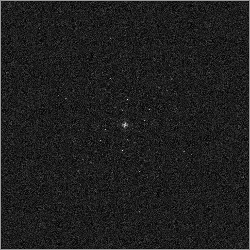
Figure 2: FFT of the example image

Using the mouse-wheel or the keys K/L to zoom, the contrast of the Fourier transform is still somewhat bad, this can be fixed by selecting a small region around a peak (using the left mouse button), and then pressing N again - the viewer will maximize contrast for the pixels contained within the selected subregion.

Now its time to add the lattice overlay, which is a 2-step process: a lattice overlay object is first created and then added to the viewer. Since the code that will be used from this point on uses the iplt module and its GUI components, we need to import the proper modules before anything else:

# import the iplt module and the iplt.gui
import iplt
import iplt.gui
# create lattice overlay
lov=iplt.gui.LatticeOverlay()
# add newly created overlay to viewer
v.AddOverlay(lov)

The result is shown on the left side of the figure 3. Note that upon editing the lattice, a new one appears in a different color (as shown on the right), while the old one remains as it is. In order to fix the new lattice, use CTRL F, and to revert back to the old one use CTRL R.

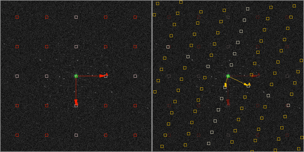
Figure 3: FFT with overlayd lattice

The following functionality is now available to to fit the lattice to the underlying pattern:

CTRL LMB

Will shift the targeted lattice point around, adjusting the remaining lattice on the fly

CTRL 2

Will fix the targeted lattice point, and subsequent adjustment of the lattice takes this constraint into account. To remove such a fixed point, press CTRL 2 while hovering with the mouse between lattice points.

CTRL G

Attempts to perform a local 2D gaussian fitting based on the underlying image, for the lattice point that the mouse is targetting

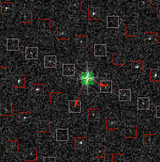
Figure 4: FFT with overlayd fitted lattice