Fourier Peak Filtering and Correlation Averaging in Iplt

The goal of this exercise is to Fourier peak filter an image of a negatively stained crystal and to further improve the average by correlation averaging.

Starting the Tutorial

First download the sample image raw.tif used in the tutorial.

• Linux: Start the tutorial with the command giplt_corr_avg (part of the iplt distribution).
• Mac OS X: Double click the IPLT Correlation Averaging icon in the Applications folder.

This will start iplt and display the list of commands used for this tutorial.

Loading the Image

Press “Load raw image” to display a dialog where you can enter the name of the inital image (raw.tif) and the pixel sampling (8 Angstroem). The pixel sampling defines the pixel dimension, i.e. 8 means that the pixel extends 8 Angstroem in x and y direction.

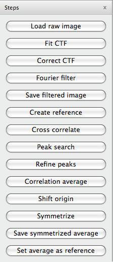
Figure 1: List of commands

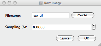
Figure 2: Load raw image dialog

You should now see two data viewers displaying the inital image and its Fourier transform. The Fourier transform will be mostly black with one bright pixel in the center. To improve the display of the Fourier transform select an area not containing the center with the mouse and press N to renormalize the image. By renormalizing the Fourier transfrom you will just modify the display of the image, not the original data.

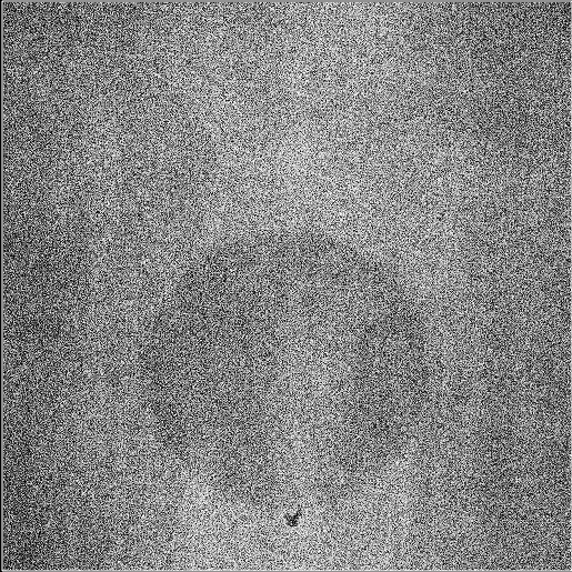
Figure 3: initial image

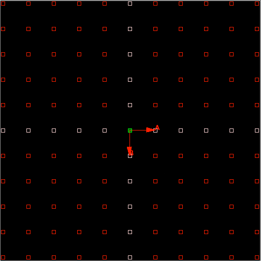
Figure 4: Fourier transform

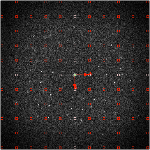
Figure 5: Renormalized image

Lattice Indexing

In the Fourier transform you see peaks corresponding to two crystal lattices. We will now fit one of the two lattices manually. Modify the Lattice Overlay (Press Control and use the LMB, CMB and RMB) to fit as well as possible one of the lattices you see in the Fourier Transform:

Control-LMB	Move Lattice Point
Control-CMB	Rotate Lattice
Control-RMB	Shift Origin
Control-1	Set first anchor
Control-2	Set second anchor
Control-F	fix new lattice
Control-R	reject new lattice

On MacOS X use Command-<key> instead of Control-<key>.

As soon as you start modifying the lattice, you will see two lattices displayed: One in red and one in beige. The lattice in red is the last saved lattice, the beige lattice is the modified version. You can go back to the red lattice by pressing <Control>+<r>. When you are satisfied with your lattice, press <Control>+<f>. This will save your new lattice. Note that for the subsequent Fourier peak filtering step, the red lattice will be used.

Example of one fitted lattice:

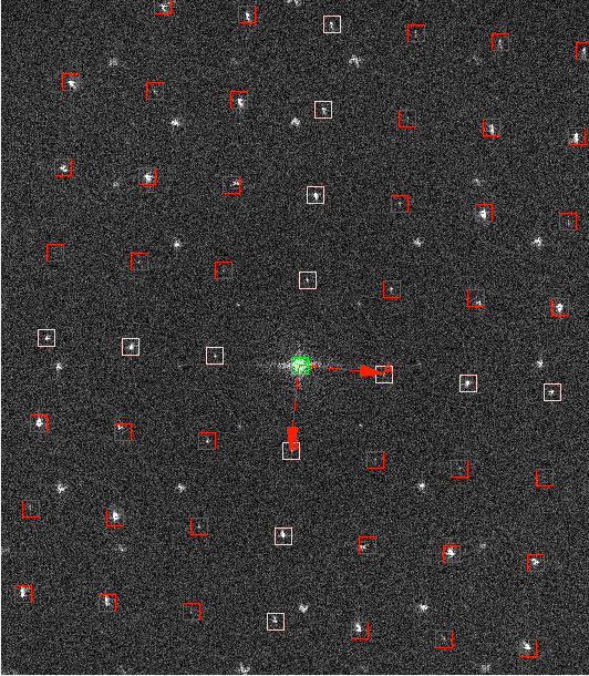
Figure 6: Manually fitted lattice

Fourier Peak Filtering

Since we know that all the information of the unit cell is concentrated on the spots in the lattice and everything outside is noise, we can now filter the image with a “Fourier Peak Filter”. On a perfect crystal, the information would be concentrated on a single pixel. However, due to crystalline imperfections (bending, crystal is not infinite in size), the information is spread out over several pixels. That’s why we include not only the central pixel of the lattice but also pixel inside a certain radius.

Press “Fourier Filtering” to Fourier peak filter the Fourier transform. A dialog will pop up to ask for the radius of the mask and for the high and low frequency cutoff values for the subsequent bandpass filter. For this example a mask radius of 5 pixels and a highpass threshold cutoff of 200 Angstroem should be reasonable. For the lowpass threshold cutoff a value of 16 Angstroem should be chosen. The dialog also asks which types of mask and of Fourier filter should be used. For both, Gaussian type should be selected.. After filtering the filtered, backtransformed image will be displayed. The red box indicates the size of a single unit cell.

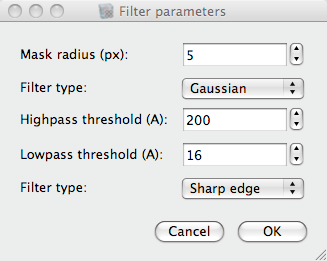
Figure 7: Fourier peak filtering dialog

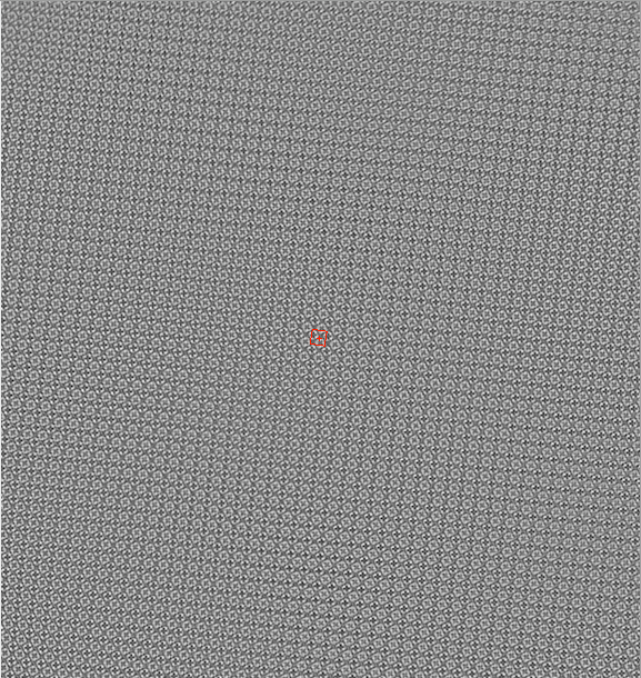
Figure 8: Fourier peak filtered image

Saving the filtered image

It is now possible to save the filtered image. This step is not necessary for further processing.

Correlation Averaging

The Correlation Averaging technique combines Fourier filtering and averaging. In the previous step, we created a Fourier filtered image which will serve us now as a reference for a cross-correlation with the original image: In combination with a peak search this will give us the locations of the unit cells of the lattice.

Select an area the size of ca. 2x2 unit cells of the filtered image with the mouse in the viewer to use it as reference. Press “Crosscorrelate” to calculate the cross correlation between inital image and selected reference. the crosscorrelation image will be displayed with the real space lattice overlayed in red.

Figure 9: Cross correlation image

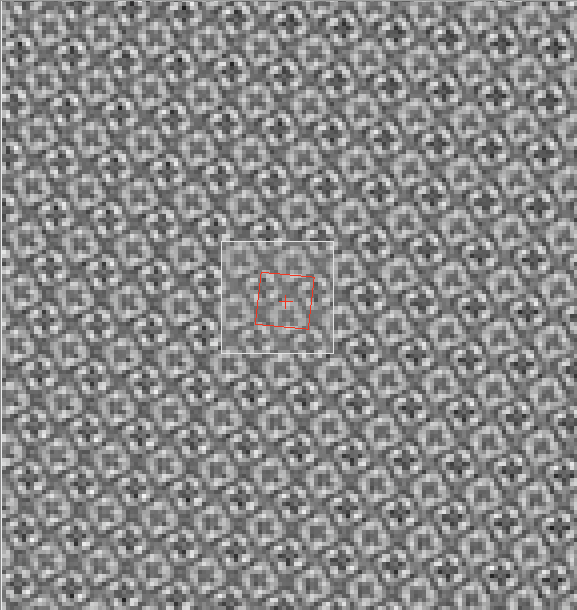
Figure 10: Selected reference

Peak search

The lattice coincides only with part of the cross correlation maxima. The reason for this are bends in the crystal lattice. With a peaksearch we can never the less find the correct position of every good unit cell and use this position information to average the unit cells. Press “Peak Search” to open the dialog for entering the peak search parameters. The outer radius gives the minimal distance two peaks have to be separated. 8 pixels is a reasonable value. For the inner radius (maximal radius of the peak maximum) use 3 pixels and for the sensitivity use 1.2. A lower sensitivity will lead to more spots to be picked up.

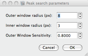
Figure 11: Peak search dialog

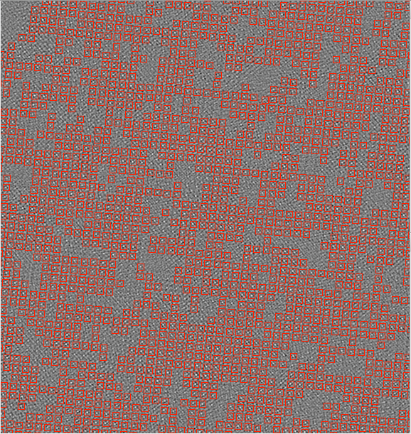
Figure 12: Cross correlation image showing the found peaks in red

If not enough or too much peaks are found, clear all the marks in the Data viewer (Display->Clear All Marks) and redo the last step with slightly different parameters.

Peak refine

The correlation peak positions can be further refined using a 2D gauss fit. For this the size of the image around a peak has to be given on which the gauss fit will be performed.

Correlation averaging

Press “Correlation average” to start the correlation averaging. A dialog will ask about the size of the final image. Depending on the number of peaks and the speed of the computer this step can take several minutes. In the end the averaged image will be displayed. The red box indicates the size of the unit cell.

Figure 13: Correlation average dialog

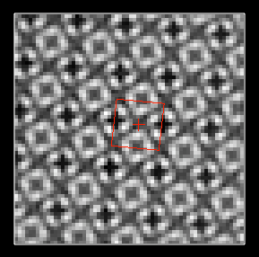
Figure 14: Correlation average

Saving the correlation average

The correlation average can now be saved by pressing “Save correlation average”.